Water Irrigation Experiment Using Microsoft Azure

Hi,

As we all know water irrigation is the foundation of global agricultural productivity, enabling farmers to buffer crops to cope with the risks of rainfall variability and drought. However, freshwater supplies to irrigated agriculture are increasingly constrained by increased demand for water from other sectors, changes in water supply due to climate change and increased awareness of the impact of irrigation on the environment.

To address these challenges, Machine learning technology plays an important role in water irrigation system. According to study by applying machine learning in agriculture it enhances the water irrigation system which helps us to use the water in efficient manner and reduces water waste.

So, In the last blog we created a model that predicts the future water requirements based on a given data using Two Class Decision Forest. Now, in today’s experiment we will try to improve our solution to get better insights of Water Irrigation system Using Microsoft Azure Machine Learning.

First, we need to collect data to build a training dataset. We choose the attributes that have significant influence on crop water usage and the data for which are available throughout the whole cropping seasons. Please note that the data we collected for this experiment was through KAISPE Agriculture Remote Monitoring solution using Azure IoT.

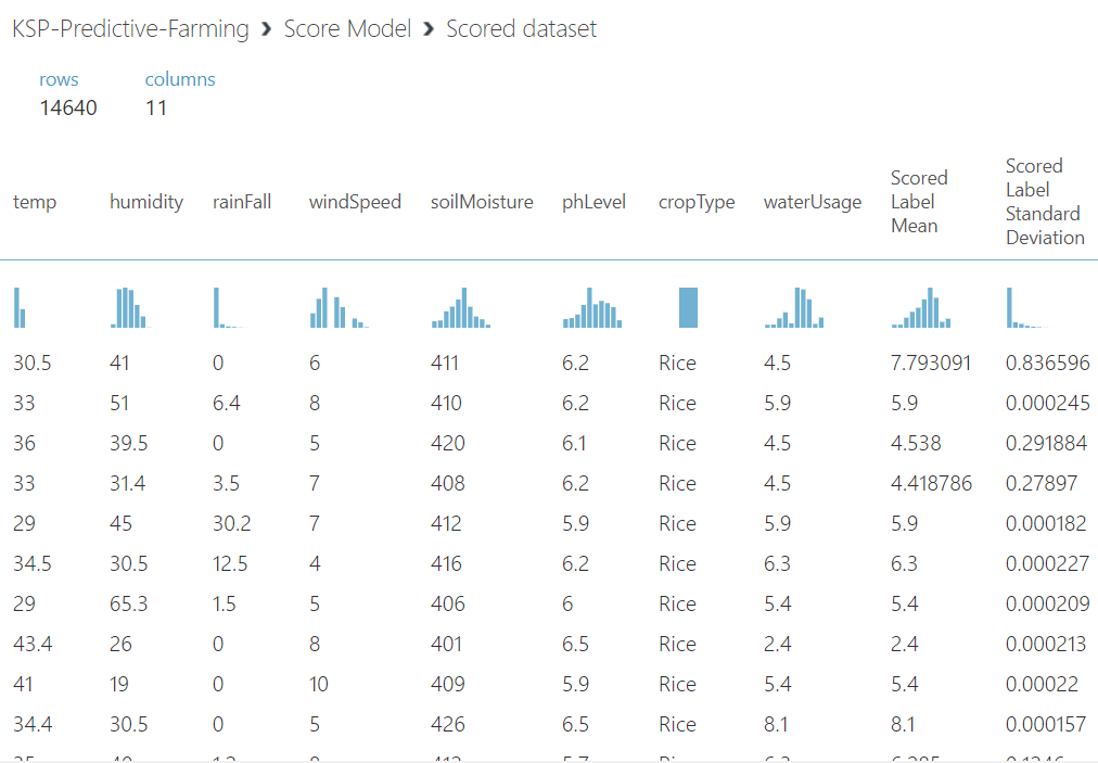
Here we have the example of a training dataset:

Our training dataset contains historical data composed of attributes on various weather parameters Temperature, Humidity, Rainfall, Wind speed, Soil Moisture, phLevel combined with Crop Type and Water Usage.

Next, the method or technique we use to predict water usage in this experiment is Decision Forest Regression. So, what is Decision Forest Regression and how decision forests work in regression tasks, lets take a look into it:

Building a number of trees called a forest, instead of a single tree. It does so in order to extract more patterns and logic rules. It basically uses the same approach of a single tree building algorithm.

Decision trees have these advantages:

They are very effective in both calculation and memory usage during training and prediction.
They can represent non-linear decision boundaries.
They perform integrated feature selection and classification, and are resilient in the presence of noisy features.

The regression model consists of a set of decision trees. Each tree in the regression decision forest outputs a Gaussian distribution as a prediction. Perform aggregation on the collection of trees to find the Gaussian distribution of the combined distribution of all the trees closest to the model. For more information: https://docs.microsoft.com/en-us/azure/machine-learning/studio-module-reference/decision-forest-regression

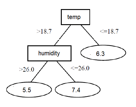
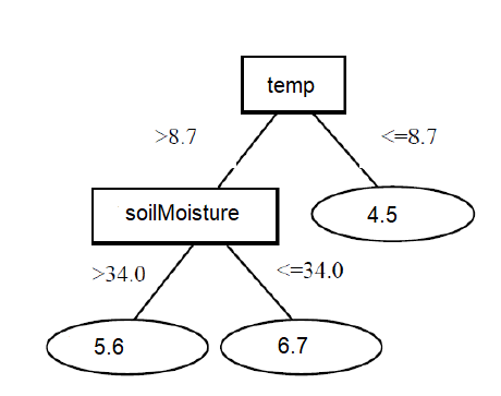
Here we have the example of a multiple decision trees from our dataset:

Now, in order to evaluate the performance of our data pre-processing techniques we build training dataset which we divide into two parts training(70%) and testing(30%). A Decision Forest Regression algorithm is applied on the training dataset, it is then applied on testing dataset to check the prediction accuracy of unseen records. Before we evaluate our model, let see the score model to see what our model has scored.

Finally, the performance of the model on the dataset is evaluated by prediction accuracy. Here we have the result that has performed the best with the accuracy of 95%.

So, if you can see the given output has Coefficient of Determination (which also known as R square) is 0.95, Mean Absolute Error is 0.07, Root Mean Squared Error is 0.28, Relative Absolute Error is 0.07 and in last Relative Squared Error which is 0.04.

For better understanding of the result lets take a look into it:

Coefficient of Determination -> It can directly indicate the excellent performance of our model. In more technical terms, we can define it as a “determination coefficient” which is a measure of the variance of the response variable “y”, which can be predicted using the predictor “x”.

Mean Absolute Error -> It is usually used when the performance is measured on continuous variable data. It gives a linear value, which averages the weighted individual differences equally. The lower the value, better is the model’s performance.

Root Mean Squared Error -> In this metric also, lower the value, better is the performance of the model.

I hope you found this blog post helpful. If you have any questions, please feel free to contact me [email protected]